9: LSTM: The basics

9: LSTM: The basics¶

In this notebook, we will learn the basics of a Long Short Term Memory (LSTM) based on Keras, a high-level API for building and training deep learning models, running on top of TensorFlow, an open source platform for machine learning.

We will build a basic LSTM to predict stock prices in the future. The data is provided in your training environment - but in future you can also access it in this github repo.

# Importing the libraries
import numpy as np
import matplotlib.pyplot as plt
import pandas as pd

from sklearn.preprocessing import MinMaxScaler

from tensorflow.keras.models import Sequential
from tensorflow.keras.layers import Dense
from tensorflow.keras.layers import LSTM
from tensorflow.keras.layers import Dropout

plt.style.use('ggplot')

Converting data to sequence structure¶

One of the critical features of $RNNs$ and $LSTMs$ is that they work on sequences of data. In the lecture notes we saw that the network takes input at a time $t$ and the hiden layer state from $t-1$ and produces an output:

However we may also want to include measured data from further back in time to help with remembering; so we could want input data from $t-1 \cdots t-n$. We might also have more than one channel of input data, this is called the window of the data. Imagine for example we were predicting stock prices, we could have the history of that stock, but we might also want to know the central bank interest rate, or the strength of one currency relative to another, in this case we have a multi-variate problem. So our input data looks more like:

Also, we might also want to make our $LSTM$ predict more than just one step forward, so we will want to be able to have multiple steps in the output.

We write a function to convert dataframe series into data that is suitable for $LSTM$ training. This function is quite flexible and can be useful in many scenarios, so it is one that you might like to reuse in future if you are training time series models.

As input we pass the data as a numpy array. We then also specify how far back in time we wish to look for each prediction n_in, so n_in = 1 means we take just $t$ as input, n_in=2 means we take $t, t-1$ as input and so on. We specify how far into the future we wish to predict, with the n_out variable. n_out=1 means we predict for $t$, n_out=2 means we predict for $t, t+1$ and so on. In addition to the window sizes, we can also select the features (columns in the data) to use with the feature_indices argument.

The series data can be infinitely long while the memory of our LSTM cannot not be infinitely large. Therefore, we need to specify the length of the LSTM, or the timesteps, which is usually much smaller than the total length of the series. The first dimension of the outputs (X and y for TensorFlow) is batch; time-dependency is ignored among the batches (i.e., they can be shuffled).

def series_to_tensorflow(data, timesteps=10, n_in=1, n_out=1, feature_indices=None):
    """
    Convert a series to tensorflow input.
    Arguments:
       data: Sequence of observations as a 2D NumPy array of shape (n_times, n_features)
       n_in: Window size of input X
       n_out: Window size of output y
       feature_indices: select features by indices; pass None to use all features
       timesteps: timesteps of LSTM
    Returns:
       X and y for tensorflow.keras.layers.LSTM
    """
    # sizes
    n_total_times, n_total_features = data.shape[0], data.shape[1]
    n_batches = n_total_times - timesteps - (n_in - 1) - (n_out - 1)
    
    # feature selection
    if feature_indices is None:
        feature_indices = list(range(n_total_features))
    
    # data
    X = np.zeros((n_batches, timesteps, n_in, len(feature_indices)), dtype='float32')
    y = np.zeros((n_batches, n_out, len(feature_indices)), dtype='float32')
    for i_batch in range(n_batches):
        for i_in in range(n_in):
            X_start = i_batch + i_in
            X[i_batch, :, i_in, :] = data[X_start:X_start + timesteps, feature_indices]
        y_start = i_batch + timesteps + n_in - 1
        y[i_batch, :, :] = data[y_start:y_start + n_out, feature_indices]
    
    # flatten the last two dimensions
    return X.reshape(n_batches, timesteps, -1), y.reshape(n_batches, -1)

A multi-variate LSTM¶

Importing and treating the data¶

We first read in our data and inspect it using pandas.

# Importing the training set
dataset_train = pd.read_csv('lstm-data/data-train-lstm.csv')

dataset_train.head()

	Date	Open	High	Low	Last	Close	Total Trade Quantity	Turnover (Lacs)
0	2018-09-28	234.05	235.95	230.20	233.50	233.75	3069914	7162.35
1	2018-09-27	234.55	236.80	231.10	233.80	233.25	5082859	11859.95
2	2018-09-26	240.00	240.00	232.50	235.00	234.25	2240909	5248.60
3	2018-09-25	233.30	236.75	232.00	236.25	236.10	2349368	5503.90
4	2018-09-24	233.55	239.20	230.75	234.00	233.30	3423509	7999.55

print(f'Dimensions of raw data: (n_times, n_features) = {dataset_train.shape}')

Dimensions of raw data: (n_times, n_features) = (2035, 8)

In the next cell, we get rid of the Date column (the first column) and normalize the rest price columns to [0, 1] using MinMaxScaler from scikit-learn.

# drop `Date` column
values = dataset_train.drop(dataset_train.columns[[0,]], axis=1).values

# normalize prices
scaler = MinMaxScaler(feature_range=(0, 1))
scaled = scaler.fit_transform(values)

print(f'Dimensions of normalized price data: (n_times, n_features) = {scaled.shape}')

Dimensions of normalized price data: (n_times, n_features) = (2035, 7)

Converting to $LSTM$ structure data¶

We now want to convert the data to a structure that can be fed to the $LSTM$. To do this we use our series_to_tensorflow function. In this case, we use 80 as the timesteps, looking back 8 steps (n_in=8) and projecting forward 4 steps (n_out=4) and considering the Open and Close prices (i.e., feature_indices=[0, 4]).

timesteps = 80
n_in = 8
n_out = 4
feature_indices = [0, 4]

X_train, y_train = series_to_tensorflow(scaled, timesteps=timesteps, 
                                        n_in=n_in, n_out=n_out, feature_indices=feature_indices)
print(f'Dimensions of X_train: (batches, timesteps, features) = {X_train.shape}')
print(f'Dimensions of y_train: (batches, features) = {y_train.shape}')

Dimensions of X_train: (batches, timesteps, features) = (1945, 80, 16)
Dimensions of y_train: (batches, features) = (1945, 8)

Building the network¶

Note that as before we start off from a Sequential type model in Keras.

The $LSTM$ layers are already coded in Keras so we do not need to worry about writing the complicated structure. We just need to consider a few hyper-parametes we want to set,

Number of LSTM layers - we can stack LSTM layers in this case we will start with 2 stacked LSTMs;
units - this is the dimensionality of the hidden state and memory cell of the LSTM;
return_sequences - should we return the full output sequence or just the final value in the sequence. Generally, if the LSTM layer is feeding to another layer in the network, this would be True; if the LSTM layer is the final layer then this is False; note default is False.

# Initialising the LSTM
regressor = Sequential()

# Adding the first LSTM layer
# shape: (N, 80, 16) => (N, 80, 50)
regressor.add(LSTM(units=50, return_sequences=True, dropout=0.4,
                   input_shape=(X_train.shape[1], X_train.shape[2])))

# Adding a second LSTM layer
# shape: (N, 80, 50) => (N, 24)
regressor.add(LSTM(units=24, return_sequences=False, dropout=0.4,))

# Adding an output layer 
# shape: (N, 24) => (N, 8)
regressor.add(Dense(units=y_train.shape[1]))

Compile the network¶

As ususal we need to compile the network, choosing an optimiser and a loss function.

We use adam as our optimiser and mean_squared_error as our loss.

# Compiling the RNN
regressor.compile(optimizer='adam', loss='mean_squared_error')

Train the network¶

# Fitting the RNN to the Training set
history = regressor.fit(X_train, y_train, epochs=30, batch_size=128)

Epoch 1/30
16/16 [==============================] - 4s 70ms/step - loss: 0.0421
Epoch 2/30
16/16 [==============================] - 1s 68ms/step - loss: 0.0093
Epoch 3/30
16/16 [==============================] - 1s 67ms/step - loss: 0.0049
Epoch 4/30
16/16 [==============================] - 1s 63ms/step - loss: 0.0036
Epoch 5/30
16/16 [==============================] - 1s 78ms/step - loss: 0.0032
Epoch 6/30
16/16 [==============================] - 1s 67ms/step - loss: 0.0030
Epoch 7/30
16/16 [==============================] - 1s 69ms/step - loss: 0.0028
Epoch 8/30
16/16 [==============================] - 1s 65ms/step - loss: 0.0028
Epoch 9/30
16/16 [==============================] - 1s 65ms/step - loss: 0.0026
Epoch 10/30
16/16 [==============================] - 1s 65ms/step - loss: 0.0025
Epoch 11/30
16/16 [==============================] - 1s 65ms/step - loss: 0.0025
Epoch 12/30
16/16 [==============================] - 1s 68ms/step - loss: 0.0026
Epoch 13/30
16/16 [==============================] - 1s 75ms/step - loss: 0.0024
Epoch 14/30
16/16 [==============================] - 1s 65ms/step - loss: 0.0025
Epoch 15/30
16/16 [==============================] - 1s 66ms/step - loss: 0.0023
Epoch 16/30
16/16 [==============================] - 1s 66ms/step - loss: 0.0022
Epoch 17/30
16/16 [==============================] - 1s 76ms/step - loss: 0.0022
Epoch 18/30
16/16 [==============================] - 1s 85ms/step - loss: 0.0022
Epoch 19/30
16/16 [==============================] - 1s 90ms/step - loss: 0.0022
Epoch 20/30
16/16 [==============================] - 1s 73ms/step - loss: 0.0022
Epoch 21/30
16/16 [==============================] - 1s 78ms/step - loss: 0.0021
Epoch 22/30
16/16 [==============================] - 1s 61ms/step - loss: 0.0020
Epoch 23/30
16/16 [==============================] - 1s 65ms/step - loss: 0.0021
Epoch 24/30
16/16 [==============================] - 1s 65ms/step - loss: 0.0021
Epoch 25/30
16/16 [==============================] - 1s 63ms/step - loss: 0.0021
Epoch 26/30
16/16 [==============================] - 1s 62ms/step - loss: 0.0020
Epoch 27/30
16/16 [==============================] - 1s 61ms/step - loss: 0.0019
Epoch 28/30
16/16 [==============================] - 1s 72ms/step - loss: 0.0021
Epoch 29/30
16/16 [==============================] - 1s 81ms/step - loss: 0.0020
Epoch 30/30
16/16 [==============================] - 1s 63ms/step - loss: 0.0019

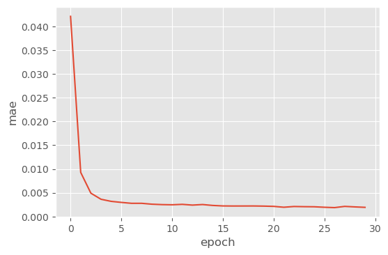
plt.figure(dpi=100)
plt.plot(history.history['loss'])
plt.xlabel('epoch')
plt.ylabel('mae')
plt.show()

Making predictions with our model¶

We now use model that we just built to predict on previously un-seen data. We read in data-test.csv and get the stock prices from that data.

# Part 3 - Making the predictions and visualising the results

# Getting the real stock price of 2017
dataset_test = pd.read_csv(data_path + 'lstm-data/data-test-lstm.csv')
real_stock_price = dataset_test.iloc[:, 1:2].values
print(dataset_test.shape)

(16, 8)

dataset_test.head()

	Date	Open	High	Low	Last	Close	Total Trade Quantity	Turnover (Lacs)
0	2018-10-24	220.10	221.25	217.05	219.55	219.80	2171956	4771.34
1	2018-10-23	221.10	222.20	214.75	219.55	218.30	1416279	3092.15
2	2018-10-22	229.45	231.60	222.00	223.05	223.25	3529711	8028.37
3	2018-10-19	230.30	232.70	225.50	227.75	227.20	1527904	3490.78
4	2018-10-17	237.70	240.80	229.45	231.30	231.10	2945914	6961.65

The testing data contain 16 time steps. We will concatenate them to the training data for time extension.

# Getting the predicted stock price of 2017
dataset_extended = pd.concat((dataset_train, dataset_test), axis=0)
values_extended = dataset_extended.drop(dataset_extended.columns[[0,]], axis=1).values
scaled_extended = scaler.transform(values_extended)
print(f'Dimensions of normalized price data: (n_times, n_features) = {scaled_extended.shape}')

Dimensions of normalized price data: (n_times, n_features) = (2051, 7)

# using the last points to generate testing data
X_test, y_test = series_to_tensorflow(scaled_extended[-(timesteps + n_in + n_out - 2 + len(dataset_test)):], 
                                      timesteps=timesteps,
                                      n_in=n_in, n_out=n_out, feature_indices=feature_indices)

# make predictions
y_pred = regressor(X_test)
print(f'Dimensions of X_test: (batches, timesteps, features) = {X_test.shape}')
print(f'Dimensions of y_test: (batches, features) = {y_test.shape}')
print(f'Dimensions of y_pred: (batches, features) = {y_pred.shape}')

Dimensions of X_test: (batches, timesteps, features) = (16, 80, 16)
Dimensions of y_test: (batches, features) = (16, 8)
Dimensions of y_pred: (batches, features) = (16, 8)

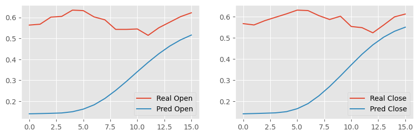
# Visualising the results
fig, ax = plt.subplots(1, len(feature_indices), dpi=100, 
                       figsize=(5 * len(feature_indices), 3), squeeze=False)
for i, index in enumerate(feature_indices):
    # we are ploting the last point from the output window
    ax[0, i].plot(y_test[:, i + (n_out - 1) * len(feature_indices)], 
                  label = 'Real ' + dataset_train.keys()[index + 1])
    ax[0, i].plot(y_pred[:, i + (n_out - 1) * len(feature_indices)], 
                  label = 'Pred ' + dataset_train.keys()[index + 1])
    ax[0, i].legend()
plt.show()

Exercise¶

Build a network with three or four $LSTM$ layers. How does this affect the performance?
Change the LSTM timesteps (timesteps) - how does a longer/shorter one affect the predictions?
Try other window sizes and features.

8: Convolutional Neural Networks

Intro to Data Analysis and Machine Learning