1: Exploratory data analysis
Contents
1: Exploratory data analysis
We start by looking at how to explore our data. We will cover
Categorical variables
Numeric variables
Looking for outliers
Exploring correlations in the data
Some extrnal resources that you might find useful:
https://towardsdatascience.com/exploratory-data-analysis-in-python-a-step-by-step-process-d0dfa6bf94ee
# data manipulation
import pandas as pd
import numpy as np

# data viz
import matplotlib.pyplot as plt
from matplotlib import rcParams
import seaborn as sns

# apply some cool styling
plt.style.use("ggplot")
rcParams['figure.figsize'] = (12,  6)

# use sklearn to import a dataset
from sklearn.datasets import load_wine
Import the data
Importing a dataset is simple with Pandas through functions dedicated to reading the data. If our dataset is a .csv file, we can just use
df = pd.read_csv("path/to/my/file.csv")
df stands for dataframe, which is Pandas’s object similar to an Excel sheet. This nomenclature is often used in the field. The read_csv function takes as input the path of the file we want to read. There are many other arguments that we can specify.
The .csv format is not the only one we can import — there are in fact many others such as Excel, Parquet and Feather.
For ease, in this example we will use Sklearn to import the wine dataset.
We eill set a new column called target which is a class for the wines.
# carichiamo il dataset
wine = load_wine()

# convertiamo il dataset in un dataframe Pandas
df = pd.DataFrame(data=wine.data, columns=wine.feature_names)
# creiamo la colonna per il target
df["target"] = wine.target
Take a quick look using Pandas
Two of the most commonly used functions in Pandas are .head() and .tail(). These two allow us to view an arbitrary number of rows (by default 5) from the beginning or end of the dataset. Very useful for accessing a small part of the dataframe quickly.
We can also use:
.shape.describe().info()
Note the .shape call is not followed by parentheses (); this is beacause shape is an attribute of the dataset, whereas describe for example is a function that acts on the dataset.
df.tail(3)
| alcohol | malic_acid | ash | alcalinity_of_ash | magnesium | total_phenols | flavanoids | nonflavanoid_phenols | proanthocyanins | color_intensity | hue | od280/od315_of_diluted_wines | proline | target | |
|---|---|---|---|---|---|---|---|---|---|---|---|---|---|---|
| 175 | 13.27 | 4.28 | 2.26 | 20.0 | 120.0 | 1.59 | 0.69 | 0.43 | 1.35 | 10.2 | 0.59 | 1.56 | 835.0 | 2 |
| 176 | 13.17 | 2.59 | 2.37 | 20.0 | 120.0 | 1.65 | 0.68 | 0.53 | 1.46 | 9.3 | 0.60 | 1.62 | 840.0 | 2 |
| 177 | 14.13 | 4.10 | 2.74 | 24.5 | 96.0 | 2.05 | 0.76 | 0.56 | 1.35 | 9.2 | 0.61 | 1.60 | 560.0 | 2 |
df.shape
(178, 14)
df.describe()
| alcohol | malic_acid | ash | alcalinity_of_ash | magnesium | total_phenols | flavanoids | nonflavanoid_phenols | proanthocyanins | color_intensity | hue | od280/od315_of_diluted_wines | proline | target | |
|---|---|---|---|---|---|---|---|---|---|---|---|---|---|---|
| count | 178.000000 | 178.000000 | 178.000000 | 178.000000 | 178.000000 | 178.000000 | 178.000000 | 178.000000 | 178.000000 | 178.000000 | 178.000000 | 178.000000 | 178.000000 | 178.000000 |
| mean | 13.000618 | 2.336348 | 2.366517 | 19.494944 | 99.741573 | 2.295112 | 2.029270 | 0.361854 | 1.590899 | 5.058090 | 0.957449 | 2.611685 | 746.893258 | 0.938202 |
| std | 0.811827 | 1.117146 | 0.274344 | 3.339564 | 14.282484 | 0.625851 | 0.998859 | 0.124453 | 0.572359 | 2.318286 | 0.228572 | 0.709990 | 314.907474 | 0.775035 |
| min | 11.030000 | 0.740000 | 1.360000 | 10.600000 | 70.000000 | 0.980000 | 0.340000 | 0.130000 | 0.410000 | 1.280000 | 0.480000 | 1.270000 | 278.000000 | 0.000000 |
| 25% | 12.362500 | 1.602500 | 2.210000 | 17.200000 | 88.000000 | 1.742500 | 1.205000 | 0.270000 | 1.250000 | 3.220000 | 0.782500 | 1.937500 | 500.500000 | 0.000000 |
| 50% | 13.050000 | 1.865000 | 2.360000 | 19.500000 | 98.000000 | 2.355000 | 2.135000 | 0.340000 | 1.555000 | 4.690000 | 0.965000 | 2.780000 | 673.500000 | 1.000000 |
| 75% | 13.677500 | 3.082500 | 2.557500 | 21.500000 | 107.000000 | 2.800000 | 2.875000 | 0.437500 | 1.950000 | 6.200000 | 1.120000 | 3.170000 | 985.000000 | 2.000000 |
| max | 14.830000 | 5.800000 | 3.230000 | 30.000000 | 162.000000 | 3.880000 | 5.080000 | 0.660000 | 3.580000 | 13.000000 | 1.710000 | 4.000000 | 1680.000000 | 2.000000 |
df.info()
<class 'pandas.core.frame.DataFrame'>
RangeIndex: 178 entries, 0 to 177
Data columns (total 14 columns):
 #   Column                        Non-Null Count  Dtype
---  ------                        --------------  -----
 0   alcohol                       178 non-null    float64
 1   malic_acid                    178 non-null    float64
 2   ash                           178 non-null    float64
 3   alcalinity_of_ash             178 non-null    float64
 4   magnesium                     178 non-null    float64
 5   total_phenols                 178 non-null    float64
 6   flavanoids                    178 non-null    float64
 7   nonflavanoid_phenols          178 non-null    float64
 8   proanthocyanins               178 non-null    float64
 9   color_intensity               178 non-null    float64
 10  hue                           178 non-null    float64
 11  od280/od315_of_diluted_wines  178 non-null    float64
 12  proline                       178 non-null    float64
 13  target                        178 non-null    int64
dtypes: float64(13), int64(1)
memory usage: 19.6 KB
Notice that info gives quite different results to describe. Info tells us about the data types - describe gives us some summary statistics.
Make names more sensible
The name od280/od315_of_diluted_wines refers to a test for protein content. But it is not very descriptive to us, let’s chance it to make life easier for ourselves later.
df.rename(columns={"od280/od315_of_diluted_wines": "protein_concentration"}, inplace=True)
Undestanding the variables
We will look at two main types of variable discussed in the lecture: categorical and numeric.
Categorical variables
Categorical variables are those where the data are labelled by class, for example it could be data on something like postcode. If we had labelled houses by postcode, then this is said to be categorical data.
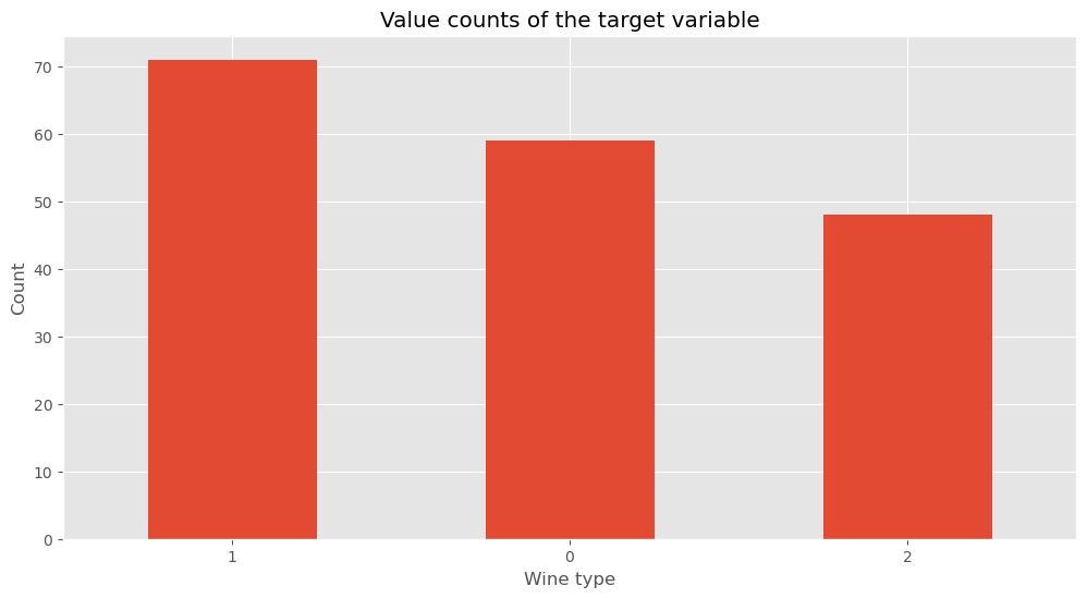
Let’s look at the distribution of the types for the wines, the target column
df.target.value_counts()
1    71
0    59
2    48
Name: target, dtype: int64
df.target.value_counts(normalize=True)
1    0.398876
0    0.331461
2    0.269663
Name: target, dtype: float64
df.target.value_counts().plot(kind="bar")
plt.title("Value counts of the target variable")
plt.xlabel("Wine type")
plt.xticks(rotation=0)
plt.ylabel("Count")
plt.show()
Numeric values
Numeric data is when we assign a numerical value as the label of an instance. To take the houses example again, we might label the houses by the distance to the nearest bus stop, this would then be a numeric data set.
We can perform exploratory analysis of the numeric values using the .describe() function.
df.magnesium.describe()
count    178.000000
mean      99.741573
std       14.282484
min       70.000000
25%       88.000000
50%       98.000000
75%      107.000000
max      162.000000
Name: magnesium, dtype: float64
df.magnesium.hist()
<AxesSubplot: >
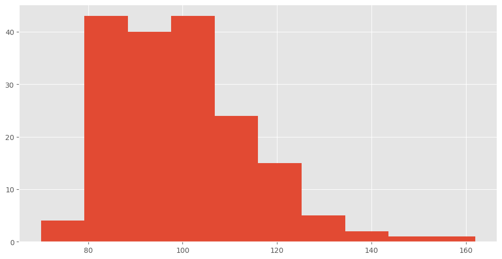
Question do you think this has high/low skew - or high/low kurotis?
print(f"Skewness: {df['magnesium'].skew()}")
print(f"Kurtosis: {df['magnesium'].kurt()}")
Skewness: 1.098191054755161
Kurtosis: 2.1049913235905557
sns.catplot(x="target", y="proline", data=df, kind="box", aspect=1.5)
plt.title("Boxplot for target vs proline")
plt.show()
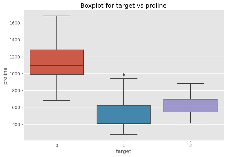
Question which of the datasets might have an outlier
sns.catplot(x="target", y="flavanoids", data=df, kind="box", aspect=1.5)
plt.title("Boxplot for target vs proline")
plt.show()
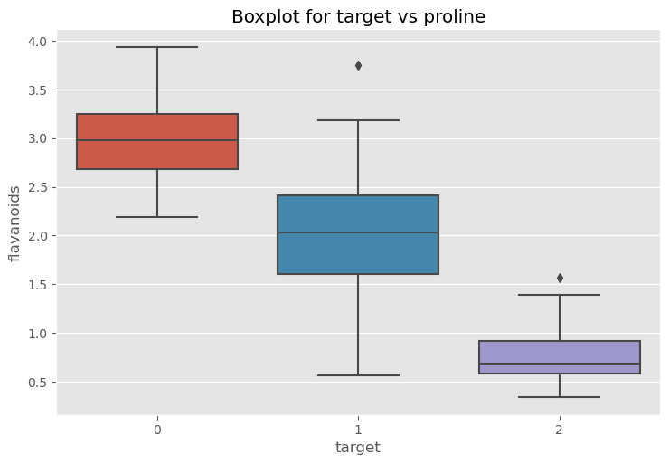
Take a closer look at the outlier
df[df['flavanoids'] > 5]
| alcohol | malic_acid | ash | alcalinity_of_ash | magnesium | total_phenols | flavanoids | nonflavanoid_phenols | proanthocyanins | color_intensity | hue | protein_concentration | proline | target | |
|---|---|---|---|---|---|---|---|---|---|---|---|---|---|---|
| 121 | 11.56 | 2.05 | 3.23 | 28.5 | 119.0 | 3.18 | 5.08 | 0.47 | 1.87 | 6.0 | 0.93 | 3.69 | 465.0 | 1 |
We can then remove that data from the data set, if we choose to.
df = df.drop(121)
Explore correlations in the data
As we discussed in the lecture we might want to remove features in the data that are very closely related to one another. Imagine a data set that had one feature with temperature in F and one with temperature in C. Now these two features tell us exactly the same thing, but on a different scale. Later we will see that adding both to a model would be of no benifit, as they do not carry any extra information. To look for redundant information between features ($x$ and $y$) we can use the correlation. $$ r = \frac{\sum(x_i - \bar{x})(y_i - \bar{y})}{\sqrt{\sum(x_i - \bar{x})^2(y_i - \bar{y})^2}} $$
corrmat = df.corr()
corrmat
| alcohol | malic_acid | ash | alcalinity_of_ash | magnesium | total_phenols | flavanoids | nonflavanoid_phenols | proanthocyanins | color_intensity | hue | protein_concentration | proline | target | |
|---|---|---|---|---|---|---|---|---|---|---|---|---|---|---|
| alcohol | 1.000000 | 0.094397 | 0.211545 | -0.310235 | 0.270798 | 0.289101 | 0.236815 | -0.155929 | 0.136698 | 0.546364 | -0.071747 | 0.072343 | 0.643720 | -0.328222 |
| malic_acid | 0.094397 | 1.000000 | 0.164045 | 0.288500 | -0.054575 | -0.335167 | -0.411007 | 0.292977 | -0.220746 | 0.248985 | -0.561296 | -0.368710 | -0.192011 | 0.437776 |
| ash | 0.211545 | 0.164045 | 1.000000 | 0.443367 | 0.286587 | 0.128980 | 0.115077 | 0.186230 | 0.009652 | 0.258887 | -0.074667 | 0.003911 | 0.223626 | -0.049643 |
| alcalinity_of_ash | -0.310235 | 0.288500 | 0.443367 | 1.000000 | -0.083333 | -0.321113 | -0.351370 | 0.361922 | -0.197327 | 0.018732 | -0.273955 | -0.276769 | -0.440597 | 0.517859 |
| magnesium | 0.270798 | -0.054575 | 0.286587 | -0.083333 | 1.000000 | 0.214401 | 0.195784 | -0.256294 | 0.236441 | 0.199950 | 0.055398 | 0.066004 | 0.393351 | -0.209179 |
| total_phenols | 0.289101 | -0.335167 | 0.128980 | -0.321113 | 0.214401 | 1.000000 | 0.864564 | -0.449935 | 0.612413 | -0.055136 | 0.433681 | 0.699949 | 0.498115 | -0.719163 |
| flavanoids | 0.236815 | -0.411007 | 0.115077 | -0.351370 | 0.195784 | 0.864564 | 1.000000 | -0.537900 | 0.652692 | -0.172379 | 0.543479 | 0.787194 | 0.494193 | -0.847498 |
| nonflavanoid_phenols | -0.155929 | 0.292977 | 0.186230 | 0.361922 | -0.256294 | -0.449935 | -0.537900 | 1.000000 | -0.365845 | 0.139057 | -0.262640 | -0.503270 | -0.311385 | 0.489109 |
| proanthocyanins | 0.136698 | -0.220746 | 0.009652 | -0.197327 | 0.236441 | 0.612413 | 0.652692 | -0.365845 | 1.000000 | -0.025250 | 0.295544 | 0.519067 | 0.330417 | -0.499130 |
| color_intensity | 0.546364 | 0.248985 | 0.258887 | 0.018732 | 0.199950 | -0.055136 | -0.172379 | 0.139057 | -0.025250 | 1.000000 | -0.521813 | -0.428815 | 0.316100 | 0.265668 |
| hue | -0.071747 | -0.561296 | -0.074667 | -0.273955 | 0.055398 | 0.433681 | 0.543479 | -0.262640 | 0.295544 | -0.521813 | 1.000000 | 0.565468 | 0.236183 | -0.617369 |
| protein_concentration | 0.072343 | -0.368710 | 0.003911 | -0.276769 | 0.066004 | 0.699949 | 0.787194 | -0.503270 | 0.519067 | -0.428815 | 0.565468 | 1.000000 | 0.312761 | -0.788230 |
| proline | 0.643720 | -0.192011 | 0.223626 | -0.440597 | 0.393351 | 0.498115 | 0.494193 | -0.311385 | 0.330417 | 0.316100 | 0.236183 | 0.312761 | 1.000000 | -0.633717 |
| target | -0.328222 | 0.437776 | -0.049643 | 0.517859 | -0.209179 | -0.719163 | -0.847498 | 0.489109 | -0.499130 | 0.265668 | -0.617369 | -0.788230 | -0.633717 | 1.000000 |
hm = sns.heatmap(corrmat,
                 cbar=True,
                 annot=True,
                 square=True,
                 fmt='.2f',
                 annot_kws={'size': 10},
                 yticklabels=df.columns,
                 xticklabels=df.columns,
                 cmap="Spectral_r")
plt.show()
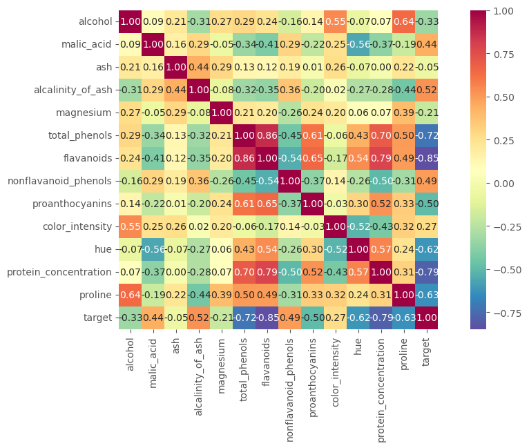
Question - which data are most correlated. If you had to choose to drop one column based on the relation to the target, which would it be? If you had to drop one of the strongly correlated columns, which would it be?