4: Linear regression
Contents
4: Linear regression
In this section we explore perhaps the simplest form of machine learnig, the venerable linear regression.
Linear regression is simply fitting models of the form
$y = mx + c$
to our data. Here, as usual, $y$ is the dependent variable, $x$ is the independent variable. $m$ is the slope of the line and $c$ the intercept.
import matplotlib.pyplot as plt
import seaborn as sns; sns.set()
import numpy as np
Fit a simple model
Let us set up some data that we want to fit. We will generate the data from a known equation:
$y = 2x + 5$
and we will add some random noise to the observed datapoints.
rng = np.random.RandomState(1)
x = 10 * rng.rand(50)
y = 2 * x - 5 + rng.randn(50)
plt.scatter(x, y)
<matplotlib.collections.PathCollection at 0x7fb378cfcd30>
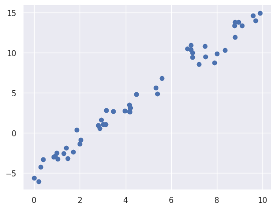
We can now use the built in LinearRegression method from scikit-learn to fit the data. Once we have fitted the data we can replot the data with the model prediction.
from sklearn.linear_model import LinearRegression
model = LinearRegression(fit_intercept=True)

model.fit(x[:, np.newaxis], y)

xfit = np.linspace(0, 10, 1000)
yfit = model.predict(xfit[:, np.newaxis])

plt.scatter(x, y)
plt.plot(xfit, yfit)
[<matplotlib.lines.Line2D at 0x7fb378cc20a0>]
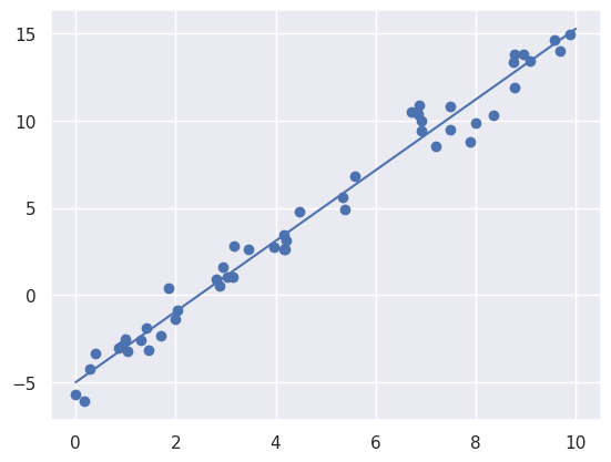
We can also look at the parameters that the model has arrived at, the slope (model.coef_[0]) and the intercept (model.intercept_). We see that the values fitted by the model are rather close to the values used to generate the data.
print("Model slope:    ", model.coef_[0])
print("Model intercept:", model.intercept_)
Model slope:     2.0272088103606953
Model intercept: -4.998577085553204
Calculate some statistics on a test set
As we saw in the section on model selection, we should always test our model on independent data, that was not used in the fitting. We generate a test set and then plot the model with the test data.
xtest = 10 * rng.rand(30)
ytest = 2 * xtest - 5 + rng.randn(30)
ypred = model.predict(xtest[:, np.newaxis])
plt.scatter(xtest, ytest)
plt.plot(xtest, ypred)
[<matplotlib.lines.Line2D at 0x7fb378ad2d60>]
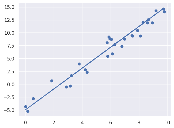
We now calculate some metrics to evaluate the model performance. Since we are doing linear regression, mean squared error, root mean squared and $r^2$ are useful metrics.
Root mean squared error may be preferred sometime to mean squared error as it gives the metric in the same units as the underlying data.
$r^2$ is often used to evaluate models - but one should exercise some caution in using $r^2$ - here is an interesting discussion of some of the limitations: Is R-squared Useless?.
We will use the metrics from scikit-learn to calculate these values between the predicted and true values of the test set.
from sklearn.metrics import mean_squared_error, r2_score

print('Mean squared error:', mean_squared_error(ypred, ytest))
print('Root mean squared error:', mean_squared_error(ypred, ytest, squared=False))
print('r-squared:', r2_score(ypred, ytest))
Mean squared error: 1.3746868656316784
Root mean squared error: 1.1724704114098907
r-squared: 0.95687909541779
Multiple linear regression
The LinearRegression estimator is much more capable than this, however—in addition to simple straight-line fits, it can also handle multidimensional linear models of the form
$y=a0+a1x1+a2x2+⋯$
where there are multiple x values. Geometrically, this is akin to fitting a plane to points in three dimensions, or fitting a hyper-plane to points in higher dimensions.
rng = np.random.RandomState(1)
X = 10 * rng.rand(100, 3)
y = 0.5 + np.dot(X, [1.5, -2., 1.])

model.fit(X, y)
print('Shape of data to fit', X.shape)
print(model.intercept_)
print(model.coef_)
Shape of data to fit (100, 3)
0.5000000000000113
[ 1.5 -2.   1. ]
Basis function regression
Here we convert our single variable $x$ to a an expression of several variables e.g. $x_1, x_2, x_3, \cdots$
This is particularly useful if you know that the relationship between the $x$ and $y$ is not linear, but you know a function (or basis) that can capture that relationship.
rng = np.random.RandomState(1)
x = 10 * rng.rand(50)
y = np.sin(x) + 0.1 * rng.randn(50)
plt.scatter(x, y)
<matplotlib.collections.PathCollection at 0x7fb378bf3190>
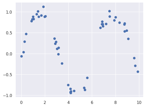
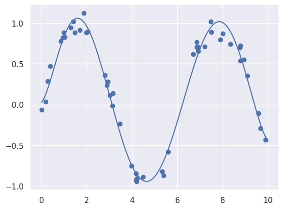
We clearly can’t fit this with a simple $y = mx + c$ - let’s try converting our $x$ into a polynomial series $x = a_0+a_1x + a_2x^2 + a_3x^3 + a_4x^4 + a_5x^5 + a_6x^6$
We can use the PolynomialFeatures class from scikit-learn - let’s put it in a pipeline, like we did before.
from sklearn.preprocessing import PolynomialFeatures
from sklearn.pipeline import make_pipeline

poly_model = make_pipeline(PolynomialFeatures(7),
                           LinearRegression())

poly_model.fit(x[:, np.newaxis], y)
yfit = poly_model.predict(xfit[:, np.newaxis])

plt.scatter(x, y)
plt.plot(xfit, yfit)
[<matplotlib.lines.Line2D at 0x7fb3786d63d0>]
xtest = 10 * rng.rand(30)
ytest = np.sin(xtest) + 0.1 * rng.randn(30)
ypred = poly_model.predict(ytest[:, np.newaxis])

print('Mean squared error:', mean_squared_error(ypred, ytest))
print('Root mean squared error:', mean_squared_error(ypred, ytest, squared=False))
print('r-squared:', r2_score(ypred, ytest))
Mean squared error: 1.2046283258545243
Root mean squared error: 1.097555614014399
r-squared: -2.461231803902191
Multiple regression
Lets try to develop a multiple linear regression model for predicting the index price from the data below
import pandas as pd

data = {'year': [2017,2017,2017,2017,2017,2017,2017,2017,2017,2017,2017,2017,2016,2016,2016,2016,2016,2016,2016,2016,2016,2016,2016,2016],
        'month': [12,11,10,9,8,7,6,5,4,3,2,1,12,11,10,9,8,7,6,5,4,3,2,1],
        'interest_rate': [2.75,2.5,2.5,2.5,2.5,2.5,2.5,2.25,2.25,2.25,2,2,2,1.75,1.75,1.75,1.75,1.75,1.75,1.75,1.75,1.75,1.75,1.75],
        'unemployment_rate': [5.3,5.3,5.3,5.3,5.4,5.6,5.5,5.5,5.5,5.6,5.7,5.9,6,5.9,5.8,6.1,6.2,6.1,6.1,6.1,5.9,6.2,6.2,6.1],
        'index_price': [1464,1394,1357,1293,1256,1254,1234,1195,1159,1167,1130,1075,1047,965,943,958,971,949,884,866,876,822,704,719]
        }

df = pd.DataFrame(data)

print(df)
    year  month  interest_rate  unemployment_rate  index_price
0   2017     12           2.75                5.3         1464
1   2017     11           2.50                5.3         1394
2   2017     10           2.50                5.3         1357
3   2017      9           2.50                5.3         1293
4   2017      8           2.50                5.4         1256
5   2017      7           2.50                5.6         1254
6   2017      6           2.50                5.5         1234
7   2017      5           2.25                5.5         1195
8   2017      4           2.25                5.5         1159
9   2017      3           2.25                5.6         1167
10  2017      2           2.00                5.7         1130
11  2017      1           2.00                5.9         1075
12  2016     12           2.00                6.0         1047
13  2016     11           1.75                5.9          965
14  2016     10           1.75                5.8          943
15  2016      9           1.75                6.1          958
16  2016      8           1.75                6.2          971
17  2016      7           1.75                6.1          949
18  2016      6           1.75                6.1          884
19  2016      5           1.75                6.1          866
20  2016      4           1.75                5.9          876
21  2016      3           1.75                6.2          822
22  2016      2           1.75                6.2          704
23  2016      1           1.75                6.1          719
We can explore the date using a pairplot to see what variables might have linear relation to index_price
import seaborn as sns
sns.pairplot(df)
<seaborn.axisgrid.PairGrid at 0x7fb3783359a0>
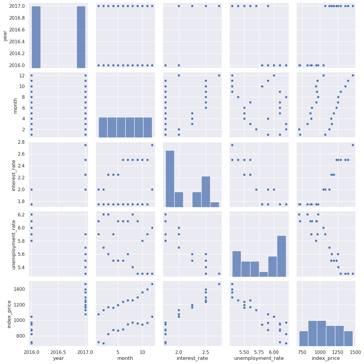
Inerest rate and unemployment rate seem to have a relationship. Month is also related somewhat, but it looks like a more complex than linear relatioship, so for now we will just use interest_rate and unemplyment as the independet variables.
Let’s now fit the multiple linear regression.
x = df[['interest_rate','unemployment_rate']]
y = df['index_price']

from sklearn.model_selection import train_test_split
# split the data with 80% in train set
xtrain, xtest, ytrain, ytest = train_test_split(x, y, random_state=0,
                                  train_size=0.5)

# with sklearn
regr = LinearRegression()
regr.fit(xtrain, ytrain)

print('Intercept: \n', regr.intercept_)
print('Coefficients: \n', regr.coef_)
Intercept:
 1141.1538024971637
Coefficients:
 [ 408.01475596 -158.2661748 ]
ypred = regr.predict(xtest)
print('Mean squared error:', mean_squared_error(ypred, ytest))
print('Root mean squared error:', mean_squared_error(ypred, ytest, squared=False))
print('r-squared:', r2_score(ypred, ytest))
Mean squared error: 7705.7212307796
Root mean squared error: 87.78223755851522
r-squared: 0.6887606394455656
We could also try individual regressions
x = df[['interest_rate']]
y = df['index_price']

# split the data with 80% in train set
xtrain, xtest, ytrain, ytest = train_test_split(x, y, random_state=0,
                                  train_size=0.5)

# with sklearn
regr = LinearRegression()
regr.fit(xtrain, ytrain)

print('Intercept: \n', regr.intercept_)
print('Coefficients: \n', regr.coef_)

ypred = regr.predict(xtest)

print('Mean squared error:', mean_squared_error(ypred, ytest))
print('Root mean squared error:', mean_squared_error(ypred, ytest, squared=False))
print('r-squared:', r2_score(ypred, ytest))
Intercept:
 -86.3608247422685
Coefficients:
 [556.16494845]
Mean squared error: 9016.89454245935
Root mean squared error: 94.95733011442218
r-squared: 0.6427482319976721
x = df[['unemployment_rate']]
y = df['index_price']

# split the data with 80% in train set
xtrain, xtest, ytrain, ytest = train_test_split(x, y, random_state=0,
                                  train_size=0.5)

# with sklearn
regr = LinearRegression()
regr.fit(xtrain, ytrain)

print('Intercept: \n', regr.intercept_)
print('Coefficients: \n', regr.coef_)

ypred = regr.predict(xtest)

print('Mean squared error:', mean_squared_error(ypred, ytest))
print('Root mean squared error:', mean_squared_error(ypred, ytest, squared=False))
print('r-squared:', r2_score(ypred, ytest))
Intercept:
 4313.884991374354
Coefficients:
 [-557.71707878]
Mean squared error: 10860.733717500003
Root mean squared error: 104.21484403625044
r-squared: 0.5585616641154836
We can see that the r-squared with multiple regression is better than either of the individual regressions.