7: Multi-layer Perceptrons
Contents
7: Multi-layer Perceptrons
In this notebook, we will learn the basics of a Deep Neural Network (DNN) based on Keras, a high-level API for building and training deep learning models, running on top of TensorFlow, an open source platform for machine learning.
We will use the fashion-mnist dataset, which is useful for quick examples when learning the basics. In DNN_practical.ipynb, we will follow the same principles to practice with a more relevant scientific dataset. To understand how a DNN works, we will implement a fully connected DNN from scratch in DNN_backprop.ipynb,
# tensorflow
import tensorflow as tf
from tensorflow import keras
from tensorflow.keras.models import Sequential
from tensorflow.keras.layers import Dense, Flatten, Dropout

# check version
print('Using TensorFlow v%s' % tf.__version__)
acc_str = 'accuracy' if tf.__version__[:2] == '2.' else 'acc'

# helpers
import numpy as np
import matplotlib.pyplot as plt
plt.style.use('ggplot')
Using TensorFlow v2.3.1
The dataset
To start with, we load the fashion-mnist dataset from Keras:
# load dataset
fashion_mnist = keras.datasets.fashion_mnist
(train_images, train_labels), (test_images, test_labels) = fashion_mnist.load_data()
# normalise images
train_images = train_images / 255.0
test_images = test_images / 255.0
# string labels
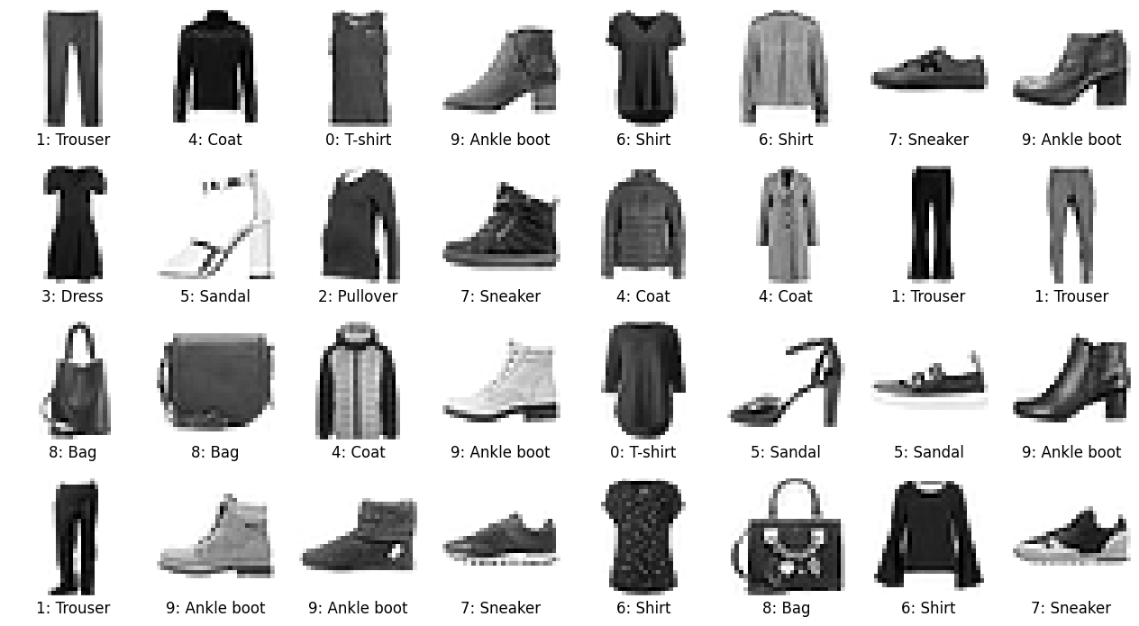
string_labels = ['T-shirt', 'Trouser', 'Pullover', 'Dress', 'Coat',
'Sandal', 'Shirt', 'Sneaker', 'Bag', 'Ankle boot']
# print info
print("Number of training data: %d" % len(train_labels))
print("Number of test data: %d" % len(test_labels))
print("Image pixels: %s" % str(train_images[0].shape))
print("Number of classes: %d" % (np.max(train_labels) + 1))
Number of training data: 60000
Number of test data: 10000
Image pixels: (28, 28)
Number of classes: 10
We can randomly plot some images and their labels:
# function to plot an image in a subplot
def subplot_image(image, label, nrows=1, ncols=1, iplot=0, label2='', label2_color='r'):
    plt.subplot(nrows, ncols, iplot + 1)
    plt.imshow(image, cmap=plt.cm.binary)
    plt.xlabel(label, c='k', fontsize=12)
    plt.title(label2, c=label2_color, fontsize=12, y=-0.33)
    plt.xticks([])
    plt.yticks([])

# ramdomly plot some images and their labels
nrows = 4
ncols = 8
plt.figure(dpi=100, figsize=(ncols * 2, nrows * 2.2))
for iplot, idata in enumerate(np.random.choice(len(train_labels), nrows * ncols)):
    label = "%d: %s" % (train_labels[idata], string_labels[train_labels[idata]])
    subplot_image(train_images[idata], label, nrows, ncols, iplot)
plt.show()
Classification by DNN
Here we will create and train a DNN model to classify the images in fashion-mnist. With Keras, the task can be divided into three essential steps:
Build the network architecture;
Compile the model;
Train the model.
These steps may be repeated for a few times to improve the quality (accuracy and stability) of the model.
1. Build the network architecture
Our first DNN will be a simple multi-layer perceptron with only one hidden layer, as shown in the following figure:
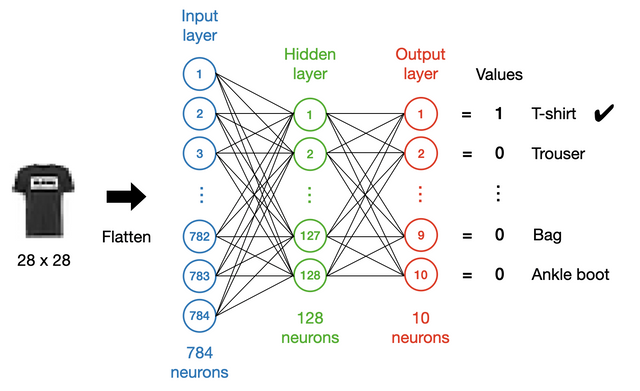
In general, a network of this kind should include an input layer, some hidden layers and an output layer. In this example, all the layers will be Dense layers.
The input layer
We first need to determine the dimensionality of the input layer. In this case, we flatten (using a Flatten layer) the images and feed them to the network. As the images are 28 $\times$ 28 in pixels, the input size will be 784.
The output layer
We usually encode categorical data as a “one-hot” vector. In this case, we have a vector of length 10 on the output side, where each element corresponds to a class of apparel. Ideally, we hope the values to be either 1 or 0, with 1 for the correct class and 0 for the others, so we use sigmoid as the activation function for the output layer:
$S(x) = \dfrac{1}{1 + e^{-x}}$
# build the network architecture
model = Sequential()
model.add(Flatten(input_shape=(28, 28)))
model.add(Dense(128, activation='relu'))
model.add(Dense(10, activation='sigmoid'))
We can take a look at the summary of the model using model.summary(). The number of trainable parameters of a layer = $P\times N+N$, where $P$ is the size of its precedent layer and $N$ its own size. Here $P\times N$ accounts for the weights of the $P\times N$ connections and $N$ for the biases of this layer.
# print summary
model.summary()
Model: "sequential"
_________________________________________________________________
Layer (type)                 Output Shape              Param #
=================================================================
flatten (Flatten)            (None, 784)               0
_________________________________________________________________
dense (Dense)                (None, 128)               100480
_________________________________________________________________
dense_1 (Dense)              (None, 10)                1290
=================================================================
Total params: 101,770
Trainable params: 101,770
Non-trainable params: 0
_________________________________________________________________
2. Compile the model
Next, we need to compile our model. This is where we specify all sorts of hyperparameters associated with the model. Here are the most important ones:
Loss
The loss is the objective function to be minimised during training. Gradients of the loss with respect to the model parameters, calculated by backpropagating the errors, determine the direction to update the model parameters. Follow DNN_backprop.ipynb to learn the details about backpropagation and gradient descent. In this case, we will use SparseCategoricalCrossentropy as the loss. The term sparse means that the output vector is sparse, with many more zeros than ones in the one-hot encoding.
Optimiser
An optimiser is an algorithm determining how the model parameters are updated based on the loss. One critical hyperparameter for the optimiser is the learning rate, which determines the magnitude to update the model parameters (also see DNN_backprop.ipynb for details). In many applications, Adam is usually a good choice at the beginning. We will use Adam in this example.
Metric
The metrics do not affect the training result but monitor the training process to give us a sense of how well the model is improving after seeing more data. We can also use them to choose between models at the end. In our case, we will monitor the accuracy.
# compile the model
model.compile(optimizer='adam',
              loss=keras.losses.SparseCategoricalCrossentropy(),
              metrics=['accuracy'])
3. Train the model
Now we can start to train the model with fashion-mnist. This is done by calling the model.fit() method, where we need to specify a few more parameters:
Epochs
It is the number of times that the model will run through the entire dataset during training.
Batch size
It determines how many data will be used at a time to determine the gradient used for parameter update. Follow DNN_backprop.ipynb to learn more about Batch, Mini-batch and Stochastic Gradient Descent.
Validation data
Accuracy and loss can be computed and logged with a validation dataset passed to model.fit(). To make predictions with a confidence equivalent to that for training, the accuracy for the validation data should not differ too much from that for the training data.
# train the model
training_history = model.fit(train_images, train_labels, epochs=50, batch_size=32,
                             validation_data=(test_images, test_labels))
Epoch 1/50
1875/1875 [==============================] - 3s 2ms/step - loss: 0.5219 - accuracy: 0.8215 - val_loss: 0.4480 - val_accuracy: 0.8476
Epoch 2/50
1875/1875 [==============================] - 3s 2ms/step - loss: 0.3864 - accuracy: 0.8620 - val_loss: 0.3906 - val_accuracy: 0.8601
Epoch 3/50
1875/1875 [==============================] - 3s 2ms/step - loss: 0.3477 - accuracy: 0.8755 - val_loss: 0.3682 - val_accuracy: 0.8705
Epoch 4/50
1875/1875 [==============================] - 3s 2ms/step - loss: 0.3230 - accuracy: 0.8826 - val_loss: 0.3696 - val_accuracy: 0.8642
Epoch 5/50
1875/1875 [==============================] - 3s 1ms/step - loss: 0.3012 - accuracy: 0.8898 - val_loss: 0.3884 - val_accuracy: 0.8614
Epoch 6/50
1875/1875 [==============================] - 3s 2ms/step - loss: 0.2852 - accuracy: 0.8944 - val_loss: 0.3630 - val_accuracy: 0.8745
Epoch 7/50
1875/1875 [==============================] - 3s 1ms/step - loss: 0.2744 - accuracy: 0.8988 - val_loss: 0.3708 - val_accuracy: 0.8689
Epoch 8/50
1875/1875 [==============================] - 2s 1ms/step - loss: 0.2631 - accuracy: 0.9028 - val_loss: 0.3444 - val_accuracy: 0.8768
Epoch 9/50
1875/1875 [==============================] - 2s 1ms/step - loss: 0.2535 - accuracy: 0.9065 - val_loss: 0.3556 - val_accuracy: 0.8731
Epoch 10/50
1875/1875 [==============================] - 2s 1ms/step - loss: 0.2461 - accuracy: 0.9089 - val_loss: 0.3567 - val_accuracy: 0.8752
Epoch 11/50
1875/1875 [==============================] - 2s 1ms/step - loss: 0.2372 - accuracy: 0.9114 - val_loss: 0.3363 - val_accuracy: 0.8815
Epoch 12/50
1875/1875 [==============================] - 2s 1ms/step - loss: 0.2289 - accuracy: 0.9148 - val_loss: 0.3333 - val_accuracy: 0.8861
Epoch 13/50
1875/1875 [==============================] - 2s 1ms/step - loss: 0.2231 - accuracy: 0.9160 - val_loss: 0.3538 - val_accuracy: 0.8773
Epoch 14/50
1875/1875 [==============================] - 2s 1ms/step - loss: 0.2170 - accuracy: 0.9186 - val_loss: 0.3593 - val_accuracy: 0.8778
Epoch 15/50
1875/1875 [==============================] - 2s 1ms/step - loss: 0.2101 - accuracy: 0.9207 - val_loss: 0.3435 - val_accuracy: 0.8851
Epoch 16/50
1875/1875 [==============================] - 3s 1ms/step - loss: 0.2041 - accuracy: 0.9238 - val_loss: 0.3540 - val_accuracy: 0.8815
Epoch 17/50
1875/1875 [==============================] - 2s 1ms/step - loss: 0.2015 - accuracy: 0.9255 - val_loss: 0.3457 - val_accuracy: 0.8851
Epoch 18/50
1875/1875 [==============================] - 3s 2ms/step - loss: 0.1957 - accuracy: 0.9268 - val_loss: 0.3489 - val_accuracy: 0.8858
Epoch 19/50
1875/1875 [==============================] - 3s 2ms/step - loss: 0.1910 - accuracy: 0.9285 - val_loss: 0.3506 - val_accuracy: 0.8904
Epoch 20/50
1875/1875 [==============================] - 2s 1ms/step - loss: 0.1838 - accuracy: 0.9310 - val_loss: 0.3598 - val_accuracy: 0.8869
Epoch 21/50
1875/1875 [==============================] - 2s 1ms/step - loss: 0.1805 - accuracy: 0.9326 - val_loss: 0.3565 - val_accuracy: 0.8876
Epoch 22/50
1875/1875 [==============================] - 3s 1ms/step - loss: 0.1776 - accuracy: 0.9331 - val_loss: 0.3485 - val_accuracy: 0.8869
Epoch 23/50
1875/1875 [==============================] - 2s 1ms/step - loss: 0.1731 - accuracy: 0.9351 - val_loss: 0.3727 - val_accuracy: 0.8784
Epoch 24/50
1875/1875 [==============================] - 3s 1ms/step - loss: 0.1706 - accuracy: 0.9359 - val_loss: 0.3765 - val_accuracy: 0.8860
Epoch 25/50
1875/1875 [==============================] - 3s 1ms/step - loss: 0.1650 - accuracy: 0.9381 - val_loss: 0.3844 - val_accuracy: 0.8832
Epoch 26/50
1875/1875 [==============================] - 2s 1ms/step - loss: 0.1623 - accuracy: 0.9396 - val_loss: 0.3677 - val_accuracy: 0.8886
Epoch 27/50
1875/1875 [==============================] - 2s 1ms/step - loss: 0.1588 - accuracy: 0.9412 - val_loss: 0.3813 - val_accuracy: 0.8864
Epoch 28/50
1875/1875 [==============================] - 2s 1ms/step - loss: 0.1556 - accuracy: 0.9412 - val_loss: 0.3980 - val_accuracy: 0.8830
Epoch 29/50
1875/1875 [==============================] - 2s 1ms/step - loss: 0.1515 - accuracy: 0.9432 - val_loss: 0.3953 - val_accuracy: 0.8863
Epoch 30/50
1875/1875 [==============================] - 3s 1ms/step - loss: 0.1489 - accuracy: 0.9444 - val_loss: 0.3905 - val_accuracy: 0.8889
Epoch 31/50
1875/1875 [==============================] - 3s 1ms/step - loss: 0.1458 - accuracy: 0.9453 - val_loss: 0.3947 - val_accuracy: 0.8856
Epoch 32/50
1875/1875 [==============================] - 3s 1ms/step - loss: 0.1444 - accuracy: 0.9448 - val_loss: 0.4130 - val_accuracy: 0.8866
Epoch 33/50
1875/1875 [==============================] - 3s 1ms/step - loss: 0.1400 - accuracy: 0.9473 - val_loss: 0.4122 - val_accuracy: 0.8824
Epoch 34/50
1875/1875 [==============================] - 4s 2ms/step - loss: 0.1379 - accuracy: 0.9481 - val_loss: 0.4118 - val_accuracy: 0.8885
Epoch 35/50
1875/1875 [==============================] - 4s 2ms/step - loss: 0.1346 - accuracy: 0.9494 - val_loss: 0.3933 - val_accuracy: 0.8913
Epoch 36/50
1875/1875 [==============================] - 3s 1ms/step - loss: 0.1324 - accuracy: 0.9501 - val_loss: 0.4290 - val_accuracy: 0.8835
Epoch 37/50
1875/1875 [==============================] - 3s 2ms/step - loss: 0.1295 - accuracy: 0.9514 - val_loss: 0.4353 - val_accuracy: 0.8884
Epoch 38/50
1875/1875 [==============================] - 4s 2ms/step - loss: 0.1303 - accuracy: 0.9511 - val_loss: 0.4043 - val_accuracy: 0.8904
Epoch 39/50
1875/1875 [==============================] - 3s 2ms/step - loss: 0.1246 - accuracy: 0.9526 - val_loss: 0.4080 - val_accuracy: 0.8896
Epoch 40/50
1875/1875 [==============================] - 3s 2ms/step - loss: 0.1237 - accuracy: 0.9531 - val_loss: 0.4116 - val_accuracy: 0.8908
Epoch 41/50
1875/1875 [==============================] - 3s 2ms/step - loss: 0.1201 - accuracy: 0.9549 - val_loss: 0.4313 - val_accuracy: 0.8873
Epoch 42/50
1875/1875 [==============================] - 3s 2ms/step - loss: 0.1185 - accuracy: 0.9558 - val_loss: 0.4455 - val_accuracy: 0.8848oss: 0.118
Epoch 43/50
1875/1875 [==============================] - 3s 1ms/step - loss: 0.1174 - accuracy: 0.9564 - val_loss: 0.4593 - val_accuracy: 0.8866
Epoch 44/50
1875/1875 [==============================] - 4s 2ms/step - loss: 0.1158 - accuracy: 0.9566 - val_loss: 0.4271 - val_accuracy: 0.8904
Epoch 45/50
1875/1875 [==============================] - 3s 2ms/step - loss: 0.1140 - accuracy: 0.9568 - val_loss: 0.4320 - val_accuracy: 0.8902
Epoch 46/50
1875/1875 [==============================] - 4s 2ms/step - loss: 0.1105 - accuracy: 0.9585 - val_loss: 0.4645 - val_accuracy: 0.8853
Epoch 47/50
1875/1875 [==============================] - 4s 2ms/step - loss: 0.1110 - accuracy: 0.9575 - val_loss: 0.4445 - val_accuracy: 0.8926
Epoch 48/50
1875/1875 [==============================] - 4s 2ms/step - loss: 0.1071 - accuracy: 0.9599 - val_loss: 0.4596 - val_accuracy: 0.8850
Epoch 49/50
1875/1875 [==============================] - 4s 2ms/step - loss: 0.1088 - accuracy: 0.9593 - val_loss: 0.4465 - val_accuracy: 0.8919
Epoch 50/50
1875/1875 [==============================] - 4s 2ms/step - loss: 0.1053 - accuracy: 0.9604 - val_loss: 0.4658 - val_accuracy: 0.8922
Check training history
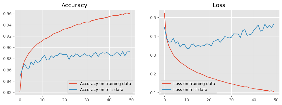
We can examine the training history by plotting accuracy and loss against epoch for both the training and the test data.
Notice that the accuracies for the training and the test data diverge as the model trains. This is a classic symptom of overfitting, that is, our model corresponds too closely to the training data so that it cannot fit the test data with an equivalent accuracy.
# plot accuracy
plt.figure(dpi=100, figsize=(12, 4))
plt.subplot(1, 2, 1)
plt.plot(training_history.history[acc_str], label='Accuracy on training data')
plt.plot(training_history.history['val_' + acc_str], label='Accuracy on test data')
plt.legend()
plt.title("Accuracy")

# plot loss
plt.subplot(1, 2, 2)
plt.plot(training_history.history['loss'], label='Loss on training data')
plt.plot(training_history.history['val_loss'], label='Loss on test data')
plt.legend()
plt.title("Loss")
plt.show()
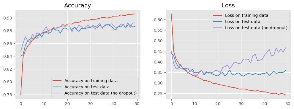
4. Regularise and re-train
Dropout, also called dilution, is a regularisation technique to mitigate against overfitting by randomly omitting a certain amount of neurons from a layer. Here we will rebuild our model with Dropout between the hidden and the output layers. Let us see whether this can negate the overfitting or not.
# build the network architecture
model_reg = Sequential()
model_reg.add(Flatten(input_shape=(28, 28)))
model_reg.add(Dense(128, activation='relu'))
model_reg.add(Dropout(0.4))
model_reg.add(Dense(10, activation='sigmoid'))

# compile the model
model_reg.compile(optimizer='adam',
                  loss=keras.losses.SparseCategoricalCrossentropy(),
                  metrics=['accuracy'])
# train the model
training_history_reg = model_reg.fit(train_images, train_labels, epochs=50, batch_size=32,
                                     validation_data=(test_images, test_labels))
Epoch 1/50
1875/1875 [==============================] - 4s 2ms/step - loss: 0.6267 - accuracy: 0.7794 - val_loss: 0.4403 - val_accuracy: 0.8402
Epoch 2/50
1875/1875 [==============================] - 4s 2ms/step - loss: 0.4496 - accuracy: 0.8387 - val_loss: 0.4276 - val_accuracy: 0.8426
Epoch 3/50
1875/1875 [==============================] - 4s 2ms/step - loss: 0.4134 - accuracy: 0.8493 - val_loss: 0.3948 - val_accuracy: 0.8570
Epoch 4/50
1875/1875 [==============================] - 5s 3ms/step - loss: 0.3951 - accuracy: 0.8559 - val_loss: 0.3752 - val_accuracy: 0.8643
Epoch 5/50
1875/1875 [==============================] - 4s 2ms/step - loss: 0.3810 - accuracy: 0.8600 - val_loss: 0.3695 - val_accuracy: 0.8672
Epoch 6/50
1875/1875 [==============================] - 4s 2ms/step - loss: 0.3682 - accuracy: 0.8652 - val_loss: 0.3704 - val_accuracy: 0.8673
Epoch 7/50
1875/1875 [==============================] - 3s 2ms/step - loss: 0.3592 - accuracy: 0.8674 - val_loss: 0.3642 - val_accuracy: 0.8697
Epoch 8/50
1875/1875 [==============================] - 4s 2ms/step - loss: 0.3497 - accuracy: 0.8724 - val_loss: 0.3707 - val_accuracy: 0.8679
Epoch 9/50
1875/1875 [==============================] - 4s 2ms/step - loss: 0.3436 - accuracy: 0.8738 - val_loss: 0.3521 - val_accuracy: 0.8754
Epoch 10/50
1875/1875 [==============================] - 4s 2ms/step - loss: 0.3355 - accuracy: 0.8754 - val_loss: 0.3656 - val_accuracy: 0.8698
Epoch 11/50
1875/1875 [==============================] - 4s 2ms/step - loss: 0.3319 - accuracy: 0.8777 - val_loss: 0.3469 - val_accuracy: 0.8765
Epoch 12/50
1875/1875 [==============================] - 4s 2ms/step - loss: 0.3279 - accuracy: 0.8786 - val_loss: 0.3501 - val_accuracy: 0.8771
Epoch 13/50
1875/1875 [==============================] - 4s 2ms/step - loss: 0.3227 - accuracy: 0.8806 - val_loss: 0.3499 - val_accuracy: 0.8758
Epoch 14/50
1875/1875 [==============================] - 4s 2ms/step - loss: 0.3174 - accuracy: 0.8814 - val_loss: 0.3588 - val_accuracy: 0.8778
Epoch 15/50
1875/1875 [==============================] - 5s 2ms/step - loss: 0.3102 - accuracy: 0.8845 - val_loss: 0.3380 - val_accuracy: 0.8838
Epoch 16/50
1875/1875 [==============================] - 4s 2ms/step - loss: 0.3113 - accuracy: 0.8840 - val_loss: 0.3496 - val_accuracy: 0.8807
Epoch 17/50
1875/1875 [==============================] - 4s 2ms/step - loss: 0.3062 - accuracy: 0.8849 - val_loss: 0.3496 - val_accuracy: 0.8811
Epoch 18/50
1875/1875 [==============================] - 4s 2ms/step - loss: 0.3045 - accuracy: 0.8863 - val_loss: 0.3459 - val_accuracy: 0.8760
Epoch 19/50
1875/1875 [==============================] - 4s 2ms/step - loss: 0.2960 - accuracy: 0.8875 - val_loss: 0.3406 - val_accuracy: 0.8828
Epoch 20/50
1875/1875 [==============================] - 4s 2ms/step - loss: 0.2978 - accuracy: 0.8870 - val_loss: 0.3352 - val_accuracy: 0.8844
Epoch 21/50
1875/1875 [==============================] - 4s 2ms/step - loss: 0.2932 - accuracy: 0.8904 - val_loss: 0.3331 - val_accuracy: 0.8825
Epoch 22/50
1875/1875 [==============================] - 4s 2ms/step - loss: 0.2908 - accuracy: 0.8906 - val_loss: 0.3431 - val_accuracy: 0.8828
Epoch 23/50
1875/1875 [==============================] - 4s 2ms/step - loss: 0.2889 - accuracy: 0.8904 - val_loss: 0.3496 - val_accuracy: 0.8820
Epoch 24/50
1875/1875 [==============================] - 4s 2ms/step - loss: 0.2860 - accuracy: 0.8926 - val_loss: 0.3322 - val_accuracy: 0.8853
Epoch 25/50
1875/1875 [==============================] - 4s 2ms/step - loss: 0.2849 - accuracy: 0.8927 - val_loss: 0.3447 - val_accuracy: 0.8815
Epoch 26/50
1875/1875 [==============================] - 4s 2ms/step - loss: 0.2820 - accuracy: 0.8931 - val_loss: 0.3613 - val_accuracy: 0.8789
Epoch 27/50
1875/1875 [==============================] - 5s 2ms/step - loss: 0.2783 - accuracy: 0.8952 - val_loss: 0.3409 - val_accuracy: 0.8834
Epoch 28/50
1875/1875 [==============================] - 5s 3ms/step - loss: 0.2788 - accuracy: 0.8954 - val_loss: 0.3367 - val_accuracy: 0.8838
Epoch 29/50
1875/1875 [==============================] - 4s 2ms/step - loss: 0.2745 - accuracy: 0.8969 - val_loss: 0.3441 - val_accuracy: 0.8836
Epoch 30/50
1875/1875 [==============================] - 4s 2ms/step - loss: 0.2711 - accuracy: 0.8962 - val_loss: 0.3472 - val_accuracy: 0.8849
Epoch 31/50
1875/1875 [==============================] - 4s 2ms/step - loss: 0.2708 - accuracy: 0.8972 - val_loss: 0.3358 - val_accuracy: 0.8847
Epoch 32/50
1875/1875 [==============================] - 5s 3ms/step - loss: 0.2715 - accuracy: 0.8976 - val_loss: 0.3315 - val_accuracy: 0.8881
Epoch 33/50
1875/1875 [==============================] - 4s 2ms/step - loss: 0.2701 - accuracy: 0.8977 - val_loss: 0.3389 - val_accuracy: 0.8864
Epoch 34/50
1875/1875 [==============================] - 4s 2ms/step - loss: 0.2664 - accuracy: 0.8986 - val_loss: 0.3446 - val_accuracy: 0.8848
Epoch 35/50
1875/1875 [==============================] - 4s 2ms/step - loss: 0.2640 - accuracy: 0.8995 - val_loss: 0.3423 - val_accuracy: 0.8891
Epoch 36/50
1875/1875 [==============================] - 4s 2ms/step - loss: 0.2630 - accuracy: 0.9007 - val_loss: 0.3390 - val_accuracy: 0.8847
Epoch 37/50
1875/1875 [==============================] - 4s 2ms/step - loss: 0.2612 - accuracy: 0.9007 - val_loss: 0.3447 - val_accuracy: 0.8874
Epoch 38/50
1875/1875 [==============================] - 4s 2ms/step - loss: 0.2640 - accuracy: 0.8997 - val_loss: 0.3410 - val_accuracy: 0.8895
Epoch 39/50
1875/1875 [==============================] - 4s 2ms/step - loss: 0.2601 - accuracy: 0.9007 - val_loss: 0.3382 - val_accuracy: 0.8885
Epoch 40/50
1875/1875 [==============================] - 4s 2ms/step - loss: 0.2581 - accuracy: 0.9013 - val_loss: 0.3447 - val_accuracy: 0.8868
Epoch 41/50
1875/1875 [==============================] - 5s 3ms/step - loss: 0.2579 - accuracy: 0.9028 - val_loss: 0.3439 - val_accuracy: 0.8822
Epoch 42/50
1875/1875 [==============================] - 5s 3ms/step - loss: 0.2559 - accuracy: 0.9027 - val_loss: 0.3504 - val_accuracy: 0.8820
Epoch 43/50
1875/1875 [==============================] - 5s 3ms/step - loss: 0.2523 - accuracy: 0.9030 - val_loss: 0.3349 - val_accuracy: 0.8870
Epoch 44/50
1875/1875 [==============================] - 5s 3ms/step - loss: 0.2501 - accuracy: 0.9048 - val_loss: 0.3449 - val_accuracy: 0.8859
Epoch 45/50
1875/1875 [==============================] - 5s 3ms/step - loss: 0.2507 - accuracy: 0.9038 - val_loss: 0.3550 - val_accuracy: 0.8899
Epoch 46/50
1875/1875 [==============================] - 4s 2ms/step - loss: 0.2508 - accuracy: 0.9038 - val_loss: 0.3433 - val_accuracy: 0.8842
Epoch 47/50
1875/1875 [==============================] - 5s 3ms/step - loss: 0.2448 - accuracy: 0.9055 - val_loss: 0.3493 - val_accuracy: 0.8891
Epoch 48/50
1875/1875 [==============================] - 5s 2ms/step - loss: 0.2494 - accuracy: 0.9051 - val_loss: 0.3487 - val_accuracy: 0.8891
Epoch 49/50
1875/1875 [==============================] - 6s 3ms/step - loss: 0.2484 - accuracy: 0.9058 - val_loss: 0.3498 - val_accuracy: 0.8859
Epoch 50/50
1875/1875 [==============================] - 6s 3ms/step - loss: 0.2426 - accuracy: 0.9063 - val_loss: 0.3588 - val_accuracy: 0.8864
# plot accuracy
plt.figure(dpi=100, figsize=(12, 4))
plt.subplot(1, 2, 1)
plt.plot(training_history_reg.history[acc_str], label='Accuracy on training data')
plt.plot(training_history_reg.history['val_' + acc_str], label='Accuracy on test data')
plt.plot(training_history.history['val_' + acc_str], label='Accuracy on test data (no dropout)')
plt.legend()
plt.title("Accuracy")

# plot loss
plt.subplot(1, 2, 2)
plt.plot(training_history_reg.history['loss'], label='Loss on training data')
plt.plot(training_history_reg.history['val_loss'], label='Loss on test data')
plt.plot(training_history.history['val_loss'], label='Loss on test data (no dropout)')
plt.legend()
plt.title("Loss")
plt.show()
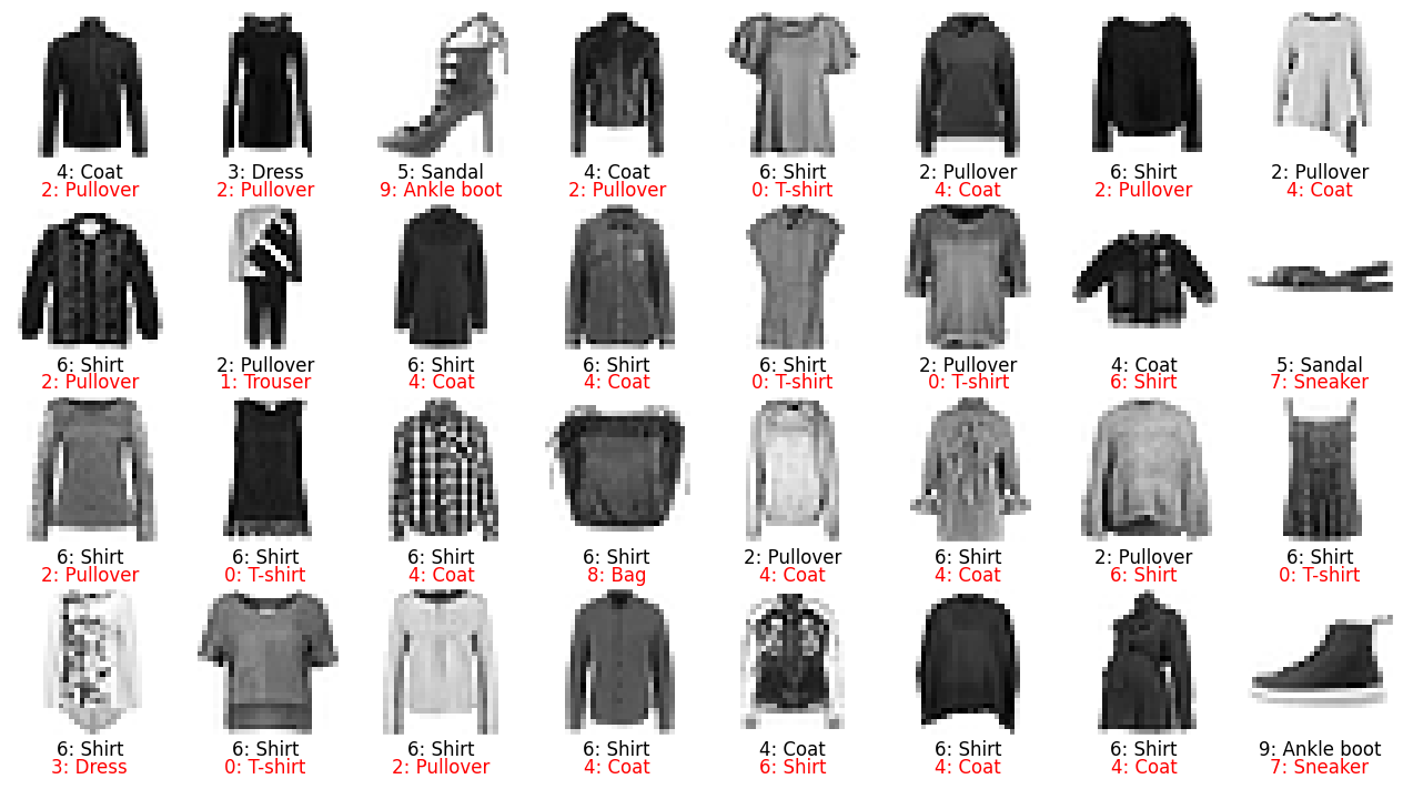
5. Make predictions
Finally, we can use our trained model to make predictions. Here we show some wrong predictions for the test data, from which we may get some ideas about what kinds of images baffle our model.
# use test images to make predictions
pred_lables = model_reg.predict(test_images).argmax(axis=1)
# get the indices of wrong predictions
id_wrong = np.where(pred_lables != test_labels)[0]
print("Number of test data: %d" % test_labels.size)
print("Number of wrong predictions: %d" % id_wrong.size)

# plot the wrong predictions
nrows = 4
ncols = 8
plt.figure(dpi=100, figsize=(ncols * 2, nrows * 2.2))
for iplot, idata in enumerate(np.random.choice(id_wrong, nrows * ncols)):
    label = "%d: %s" % (test_labels[idata], string_labels[test_labels[idata]])
    label2 = "%d: %s" % (pred_lables[idata], string_labels[pred_lables[idata]])
    subplot_image(test_images[idata], label, nrows, ncols, iplot, label2, 'r')
plt.show()
Number of test data: 10000
Number of wrong predictions: 1136
Exercises
Change some hyperparameters in
model.compile()andmodel.fit()to see their effects (see reference of tf.keras.Model);Use two hidden layers (with dropout), e.g., respectively with sizes 256 and 64, and see whether the accuracy can be improved or not;
Change the output from 0-1 binary to probability, i.e., the one-hot vector represents the probabilities that an image belongs to the classes; this can be achieved by 1) removing
activation='sigmoid'from the output layer and 2) appending aSoftmaxlayer after the trained model, e.g.,
probability_model = Sequential([model_reg, keras.layers.Softmax()])