6: Classification using decision trees

6: Classification using decision trees¶

Decision trees are one of the most popular methods from classical machine learning. They are great for situations with small data sets with structured data, such as tables of features.

Concepts covered¶

Supervised machine learning
Classical machine learning
Parameters/hyperparameters
Decision trees
Overfitting
Evaluation/metrics
Test/train split, cross-validation
Bagging and boosting

import matplotlib.pyplot as plt
from sklearn.datasets import make_blobs
import numpy as np
plt.style.use('ggplot')

Some helper functions in advance¶

This is just a function to help make some nice plots of our results.

def visualize_classifier(model, ax=None, cmap='viridis'):
    ax = ax or plt.gca()
    
    # Plot the training points
    ax.scatter(X[:, 0], X[:, 1], marker='o', c=y, s=20, cmap=cmap,
               clim=(y.min(), y.max()), zorder=3, alpha=0.7, edgecolors='black' )
    ax.axis('tight')
    ax.axis('off')
    xlim = ax.get_xlim()
    ylim = ax.get_ylim()
    
    # fit the estimator
    xx, yy = np.meshgrid(np.linspace(*xlim, num=200),
                         np.linspace(*ylim, num=200))
    Z = model.predict(np.c_[xx.ravel(), yy.ravel()]).reshape(xx.shape)

    # Create a color plot with the results
    n_classes = len(np.unique(y))
    contours = ax.contourf(xx, yy, Z, alpha=0.3,
                           levels=np.arange(n_classes + 1) - 0.5,
                           cmap=cmap, clim=(y.min(), y.max()),
                           zorder=1)

    ax.set(xlim=xlim, ylim=ylim)

Set up the data¶

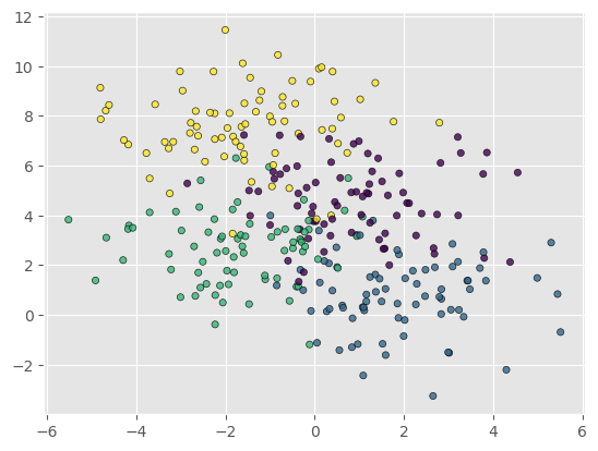
For this lecture and example we will be using a dataset of blobs that is generated automatically by scikit-learn. We generate a dataset of 300 samples with 4 different centres of the data. Use the code below to generate and plot the data.

X, y = make_blobs(n_samples=300, centers=4,
                  random_state=0, cluster_std=1.5)
plt.scatter(X[:, 0], X[:, 1], marker='o', c=y, s=20, alpha=0.8, edgecolors='black')

<matplotlib.collections.PathCollection at 0x7fafa447c2e0>

_images/lecture-5-decision-trees-classification_6_1.png

Setting up a decision tree¶

We can import a decision tree classifier from scikit-learn and use this to try to classify the data into clsuters.

Go to lecture notes to cover the theory of decision trees

Hyperparameters¶

There are many hyperparameters that can be set for the decision tree classifier. For the purposes of this tutorial we will consider only a few of these. For a full list see the DecisionTreeClassifier documentation

`max_depth`¶

The maximum depth of the tree. If None, then nodes are expanded until all leaves are pure or until all leaves contain fewer than min_samples_split samples.

`min_samples_split`¶

The minimum number of samples required to split an internal node:

* If int, then consider min_samples_split as the minimum number.
* If float, then min_samples_split is a fraction and ceil(min_samples_split * n_samples) are the minimum number of samples for each split.

`max_features`¶

The maximum number of features of the input data that can be used for splitting. If this is left as None then the max_features is the number of features.

Our model¶

For our model we will simply go with the default hyperparameters and see how the network performs.

from sklearn.tree import DecisionTreeClassifier
decision_tree = DecisionTreeClassifier()

Fit the model to our data¶

In this instance we do not need to do much feature engineering - the data that we have are relatively simple and have only two features; the coordinates on the plane.

The model objects in scikit-learn have a fit method, which takes the feature X and label y data as inputs and fits the model. Use the code below to fit the model and then use the visualize_classifier helper function to look at the result.

tree = decision_tree.fit(X, y)

visualize_classifier(tree)

/tmp/ipykernel_6938/3210908485.py:19: UserWarning: The following kwargs were not used by contour: 'clim'
  contours = ax.contourf(xx, yy, Z, alpha=0.3,

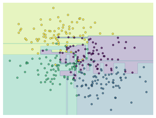
_images/lecture-5-decision-trees-classification_11_1.png

Notice that in the middle there seem to be rather arbitrary classification of regions of the data. Try rerunnig the clustering for different random sub-sets of the training data.

fig, ax = plt.subplots(1, 2, figsize=(16, 6))
fig.subplots_adjust(left=0.0625, right=0.95, wspace=0.1)
decision_tree = tree.fit(X[::2], y[::2])
visualize_classifier(tree, ax=ax[0])
decision_tree = tree.fit(X[1::2], y[1::2])
visualize_classifier(tree, ax=ax[1])

/tmp/ipykernel_6938/3210908485.py:19: UserWarning: The following kwargs were not used by contour: 'clim'
  contours = ax.contourf(xx, yy, Z, alpha=0.3,
/tmp/ipykernel_6938/3210908485.py:19: UserWarning: The following kwargs were not used by contour: 'clim'
  contours = ax.contourf(xx, yy, Z, alpha=0.3,

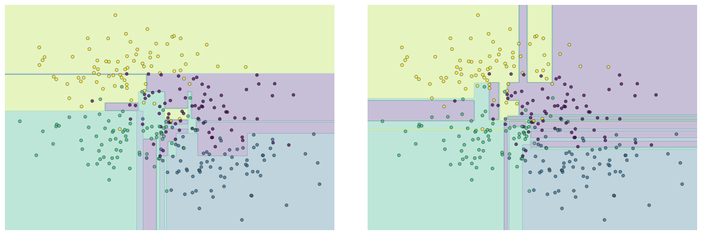
_images/lecture-5-decision-trees-classification_13_1.png

You can see that the classification is consistent in some regions, but quite different in the centre of the plot. It is concerning that the details of the classification in the centre of the plot are depedent on the training data. This is a classic sign that the model is overfitting.

Of course, we can see visually that this overfitting is occuring, but is there a more systematic way of detecting overfitting?

To do this we first need to have an objective measure of how well the model is performing. We need a metric.

Go to lecture notes to cover metrics for evaluation of models.

Evaluation¶

We are now in a position to evaluate how the model is performing. Let’s start by once again fitting the model to our dataset (X, y).

Next we get the predicted values of y by using the predict method of the new model.

Finally use the accuracy_score metric from scikit-learn to get the accuracy of the model on this data

from sklearn.metrics import accuracy_score

tree = DecisionTreeClassifier().fit(X, y)
y_pred = tree.predict(X)
print(accuracy_score(y, y_pred))

1.0

That’s pretty accurate!!

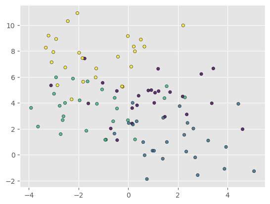
But wait up a moment - let’s try the model on some new data - generated the same way as before, but which was not used in the training.

Xnew, ynew = make_blobs(n_samples=100, centers=4,
                  random_state=0, cluster_std=1.6)
plt.scatter(Xnew[:, 0], Xnew[:, 1], marker='o', edgecolors='black', c=ynew, s=20, alpha=0.8)

<matplotlib.collections.PathCollection at 0x7faf99f85400>

_images/lecture-5-decision-trees-classification_18_1.png

y_pred = tree.predict(Xnew)
print(accuracy_score(ynew, y_pred))

0.68

That’s not quite as good as before!

The model is overfitting - i.e. it is performing well on training data but not generalising beyond the training set. This often results when the model has too many parameters and fits too flexibly to the training data. The number of parameters in the model is a hyper parameter and must be specified to choose the model.

Hyperparameter tuning and crossvalidation¶

We are going to use a training/test split and cross-validation to tune the hyper parameters of the model. Go to the lecture notes for some more in-depth examples.

Below is some code to set up a search across the max_depth parameter ranging from 1 - 20. For each value of the hyperparameter, we use a 5-fold cross validation.

from sklearn.model_selection import GridSearchCV
param_grid = {'max_depth':range(1, 20, 1)}
tree = DecisionTreeClassifier()
search = GridSearchCV(tree, param_grid, cv=5)
gs = search.fit(X, y)

plt.plot(search.cv_results_['mean_test_score'])
plt.xlabel('Tree depth')
plt.ylabel('Val Accuracy')

Text(0, 0.5, 'Val Accuracy')

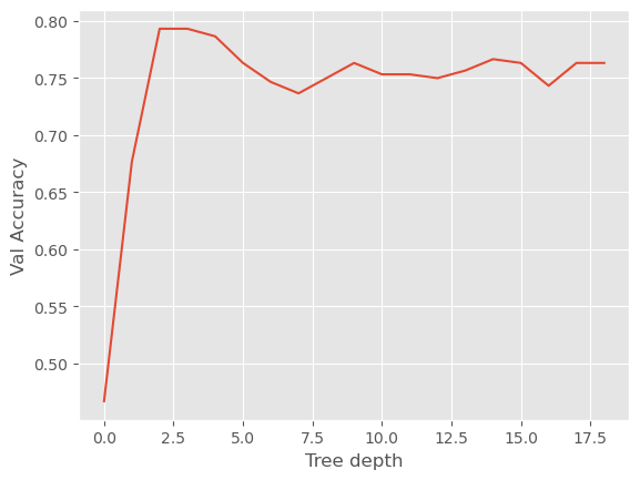
_images/lecture-5-decision-trees-classification_22_1.png

You should see that the cross-validation score has a maximum at somewhere around 3 for the max_depth. We take the best performing hyperparameter and retrain the model on the full dataset, we than apply this model to the new, unseen data and see how it performs.

depth = gs.best_params_['max_depth']
tree = DecisionTreeClassifier(max_depth=depth).fit(X, y)
y_pred = tree.predict(Xnew)
print(accuracy_score(ynew, y_pred))

0.71

Bagging and boosting¶

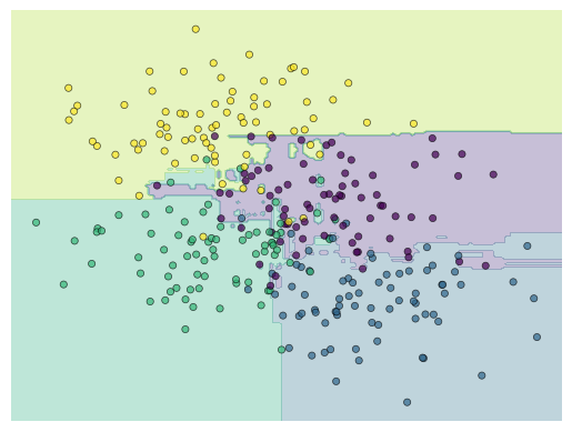
We can improve the performance of decision trees in two simple ways. Bagging and boosting. Bagging involves training an ensemble of trees on subsets of the training set. This way we can take the average result of the ensemble rather than any given individual result.

Boosting involves training a new decision tree based on the errors of the first tree. See the lecture notes for a more in depth discussion of bagging and boosting.

from sklearn.ensemble import RandomForestClassifier

forest = RandomForestClassifier(n_estimators=300, random_state=0)
model = forest.fit(X, y)
visualize_classifier(model)

/tmp/ipykernel_6938/3210908485.py:19: UserWarning: The following kwargs were not used by contour: 'clim'
  contours = ax.contourf(xx, yy, Z, alpha=0.3,

_images/lecture-5-decision-trees-classification_26_1.png

y_pred = forest.predict(Xnew)
print(accuracy_score(ynew, y_pred))

0.7

Hyperparams¶

Try to do hyperparameter tuning on the boosted decision tree to see if you can improve this result.

from sklearn.model_selection import RandomizedSearchCV

param_distributions = {
    "n_estimators": [1, 20, 50, 200, 500],
    "max_leaf_nodes": [2, 5, 10, 20, 50, 100]
}
search_cv = RandomizedSearchCV(
    forest, param_distributions=param_distributions,
    scoring="neg_mean_absolute_error", n_iter=100, random_state=0, n_jobs=2,
)
search_cv.fit(X, y.ravel())

/home/keeeto/mambaforge/envs/tf/lib/python3.8/site-packages/sklearn/model_selection/_search.py:306: UserWarning: The total space of parameters 30 is smaller than n_iter=100. Running 30 iterations. For exhaustive searches, use GridSearchCV.
  warnings.warn(

RandomizedSearchCV(estimator=RandomForestClassifier(n_estimators=300,
                                                    random_state=0),
                   n_iter=100, n_jobs=2,
                   param_distributions={'max_leaf_nodes': [2, 5, 10, 20, 50,
                                                           100],
                                        'n_estimators': [1, 20, 50, 200, 500]},
                   random_state=0, scoring='neg_mean_absolute_error')

In a Jupyter environment, please rerun this cell to show the HTML representation or trust the notebook.
On GitHub, the HTML representation is unable to render, please try loading this page with nbviewer.org.

best_forest = search_cv.best_estimator_
y_pred = best_forest.predict(Xnew)
print(accuracy_score(ynew, y_pred))

0.74

5:Naive Bayes classification

7: Multi-layer Perceptrons

Intro to Data Analysis and Machine Learning

6: Classification using decision trees

Contents

6: Classification using decision trees¶

Concepts covered¶

Some helper functions in advance¶

Set up the data¶

Setting up a decision tree¶

Hyperparameters¶

`max_depth`¶

`min_samples_split`¶

`max_features`¶

Our model¶

Fit the model to our data¶

Evaluation¶

Hyperparameter tuning and crossvalidation¶

Bagging and boosting¶

Hyperparams¶

Intro to Data Analysis and Machine Learning

6: Classification using decision trees

Contents

6: Classification using decision trees¶

Concepts covered¶

Some helper functions in advance¶

Set up the data¶

Setting up a decision tree¶

Hyperparameters¶

max_depth¶

min_samples_split¶

max_features¶

Our model¶

Fit the model to our data¶

Evaluation¶

Hyperparameter tuning and crossvalidation¶

Bagging and boosting¶

Hyperparams¶

`max_depth`¶

`min_samples_split`¶

`max_features`¶